This post assumes basic familiarity with Turing machines, P, NP, NP-completeness, decidability, and undecidability. The reader is referred to the book by Sipser, or the book by Arora and Barak for any formal definitions that have been skipped in this post. Without further ado, let’s dive in.

Introduction

Preliminaries: Search and Decision Problems

In an earlier post, we familiarised ourselves with the notion of reductions . Towards the end, we introduced the notion of self-reducibility which is our main topic of focus today. We start by familiarising ourselves with a few concepts.

In the world of complexity and computability, a language is a set of strings formed out of some alphabet. Formally, $L\subseteq {\mathrm{\Sigma }}^{\ast }$, where the alphabet $\mathrm{\Sigma }$ is a finite set of symbols, and ${\mathrm{\Sigma }}^{\ast }$ refers to the Kleene closure of $\mathrm{\Sigma }$.

Last time we formalized reductions in terms of Turing Machines . We now explicitly define mapping reductions (equivalent to Karp reductions for TMs) in terms of languages. Let $L_1\subseteq {\mathrm{\Sigma }}_1^{\ast }$ and $L_2\subseteq {\mathrm{\Sigma }}_2^{\ast }$ be languages. Recall that $L_1{\le }_m{L}_2$ (or, $L_1$ reduces to $L_2$), if there exists a computable function $f:{\mathrm{\Sigma }}_1^{\ast }\mapsto {\mathrm{\Sigma }}_2^{\ast }$ s.t. for every $w\in {\mathrm{\Sigma }}_1^{\ast }$, $w\in L_1⟺f(w)\in L_2$. We sometimes use the notation $A{\le }_m^{p}B$ to denote that the function $f$ is polynomial time constructible.

A decision problem is a Boolean-valued function $D:{\mathrm{\Sigma }}^{\ast }\mapsto \{0,1\}$. We can view $D$ as a language $L_D=\{x\in {\mathrm{\Sigma }}^{\ast }:D(x)=1\}$. Conversely, every language $L\subseteq {\mathrm{\Sigma }}^{\ast }$ can be uniquely associated with a unique decision problem $D_L$ called the membership problem. Here, $x\in L⟺D_L(x)=1$. A Turing machine $T$ computes/solves the decision problem $D$ if for any input $x\in {\mathrm{\Sigma }}^{\ast }$, $T$ halts on any input $x$ and produces output $T(x)=D(x)$.

Recall that complexity classes P and NP are defined w.r.t. decision problems. $L$ is in P if $\mathrm{\exists }$ an efficient decider for the membership problem of any string in ${\mathrm{\Sigma }}^{\ast }$. $L$ is in NP if there exists an efficient verifier and a polynomial sized certificate for the membership problem of any string in ${\mathrm{\Sigma }}^{\ast }$.

In complexity theory, many problems can be naturally expressed as search problems (for example, TSP, HamCycle, etc.), but are shoehorned into the above model of decision problems in order for us to easily classify them into classes like P and NP.

Search Problems: A search problem is a relation $R\subset {\mathrm{\Sigma }}_{in}^{\ast }\times {\mathrm{\Sigma }}_{out}^{\ast }$, i.e., $(x,y)\in R$, where $x\in {\mathrm{\Sigma }}_{in},y\in {\mathrm{\Sigma }}_{out}$ are strings belonging to the input and output alphabets respectively. Search problems are also known as relational problems / optimization problems.

A Turing machine $T$ decides/computes/solves $R$, if for any input $x\in {\mathrm{\Sigma }}_{in}$, $T(x)$ halts and produces $y\in {\mathrm{\Sigma }}_{out}$ s.t. $(x,y)\in R$, or correctly states that no such $y$ exists.

We remark here that a relation $R\subset {\mathrm{\Sigma }}_{in}^{\ast }\times {\mathrm{\Sigma }}_{out}^{\ast }$ is said to be polynomially-balanced if for any $(x,y)\in R$, $|y|=\text{poly}(|x|)$.

Since the complexity class NP is defined w.r.t. decision problems, we need to introduce an equivalent notion for search problems. Informally, this is denoted by the class FNP (or Function NP). (We make this informal connection explicit shortly.)

A relation $R$ is polynomially balanced, if for any $(x,y)\in R$, $|y|\le \mathrm{poly}(|x|)$. In other words, any certificate/witness for an instance $x$ is at most polynomially large w.r.t. $x$.

Formally, a polynomially-balanced relation $R\in$ FNP (i.e., $R$ is an NP search problem) if $R$ is polynomial-time computable.

A search problem $R$ is in FP if $R\in$ FNP and if there exists an efficient decider for $R$.

Note that FP is analogous to P in the context of search problems. The following theorem cements this analogy.

FP = FNP iff P = NP.

Search-to-Decision reductions

Recall that decision problems answer the following flavour of questions:

Given a problem $P$, is $x$ a solution to $P$? (Yes/No).

On the other hand, search problems answer the following flavour of questions:

Given a problem $P$, output a solution to $P$ (preferably with some constraints on the solution).

For example, given a problem $P$, output a solution to $P$ that has the minimum length.

We use the satisfiability problem (SAT) and its search version (FSAT) as an example to further illustrate the two notions:

• Decision problem: Given a propositional formula $\varphi$, decide if $\varphi$ is satisfiable. (SAT)
• Search problem: Given a propositional formula $\varphi$, find a satisfying assignment for $\varphi$. (FSAT)

It is straightforward to see that if it is easy to solve the Search version of a problem $P$, it is straightforward to solve the Decision version of $P$ (we can easily construct an example / counterexample!). The more challenging question is:

Can we efficiently solve the Search version of a problem $P$, if we know how to solve the Decision version of $P$ efficiently?

A problem is self-reducible or auto-reducibile if it admits an efficient search-to-decision reduction, i.e., any efficient solution to the decision version of the problem implies an efficient solution to the search version of the problem.

In this section, we see some examples of search-to-decision reductions / self-reducibility. Let us start with designing a search-to-decision reduction using SAT and FSAT, which are NP-complete and FNP-complete problems respectively.

Search-to-Decision Reduction for SAT

Formally, let $O_D^p$ be a decision oracle for a search problem $R\subset {\mathrm{\Sigma }}_{in}^{\ast }\times {\mathrm{\Sigma }}_{out}^{\ast }$ s.t. querying $O_D^p$ produces $\mathbb{I}[\mathrm{\exists }x\in {\mathrm{\Sigma }}_{in};|;x\text{ has property }p]$; i.e., querying $O_D$ with an appropriate parameter for a _property_ $p$ outputs a yes or a no indicating if there exists any input that satisfies the property $p$ (usually taken to be some bound on the input size). Our goal now is to produce $y\in {\mathrm{\Sigma }}_{out}$ s.t. $(x,y)\in R$, using oracle calls to $O_D^p$.

There are two inputs to the FSATSearchToDecision() reduction

• the propositional formula $\varphi$ or f, and
• the decision oracle for SAT on $O_D$ or DSAT(f,assign) which takes as input a propositional formula f and a restricted assignment assign and returns yes iff f is satisfiable under the restriction assign. The output of the FSATSearchToDecision() procedure is a satisfying assignment for $\varphi$( or f).

FSATSearchToDecision(f,DSAT()){
    assignarr = [*,*,....,*];// Intitalize assignarr as an n-bit empty array.
    if(DSAT(f,assignarr)=0) // is f satisfiable without restrictions?
        return -1; // f is not satisfiable
    for (i=1;i<=n; i++){
        assignarr[i]= 0
        //Fix the ith bit in x to be 1.
        // This fixes the ith literal in f.
        if (DSAT(f,assignarr)==1)
            continue;
        // move on to the i+1th coordinate,
        // with the ith bit set to 0.
        assignarr[i]= 1
        //Fix the ith bit in x to be 0.
        // This fixes the ith literal in f.
        if (DSAT(f,assignarr)==1)
            continue;
        // move on to the i+1th coordinate,
        // with the ith bit set to 1.
    return assignarr;
}

Search-to-Decision Reduction for CLIQUE

Earlier we saw that the property used by the decision oracle was a restricted assignment. We list another example of a search-to-decision reduction for the Clique problem (another one of Karp’s original 21 NP-complete problems), to give a flavour of a different decision oracle property - based on size.

• The Clique Decision problem: Given a graph $G=(V,E)$, decide if $G$ contains a clique of size $\le k$.
• The Clique Search problem: Given a graph $G=(V,E)$, find a clique of size $\le k$ in $G$ if it exists.

As seen above, there are two inputs to the CliqueSearchToDecision() reduction:

• the graph $G$ as an adjacency list L, and
• the decision oracle for Clique on $O_D$ or DCLIQUE(L,k) which takes as input a adjacency list L and a parameter k and returns yes iff the graph corresponding to L contains a clique of size at most k. The output of the CliqueSearchToDecision() procedure is an adjacency list corresponding to a clique in $G$ of size $\le k$.

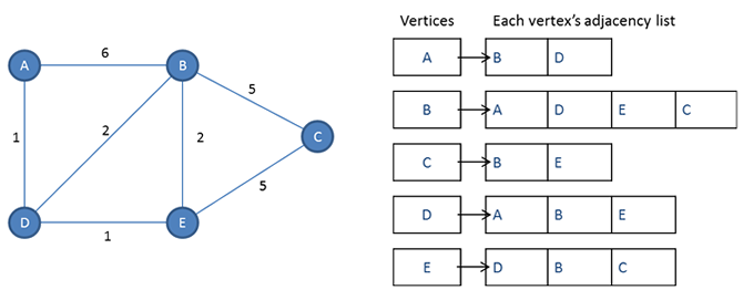
Recall that an adjacency list is a collection of unordered lists used to represent a finite graph. We use the following definition of adjacency lists (this is a modification of the definition given in CLRS): An adjacency list is a singly linked list where each element in the list corresponds to a particular vertex, and each element in the list itself points to a singly linked list of the neighboring vertices of that vertex. See the diagram below.

CliqueSearchToDecision(L,DCLIQUE()){
    if(DCLIQUE(L,k)=0)
        return -1; // There is no clique of size at most k
    for every vertex v of G {
        Let Lv be the new adjacency list
        obtained by removing vertex v from G.
        // easily done using the above datastructure.
        if(DCLIQUE(Lv,k)=1)
            L = Lv; // update the graph to reflect G = G-v.
    }
    return L;
}

Downward-self-reducibility

A related concept to self-reducibility is the notion of downward-self-reducibility. Broadly speaking, self-reducibility asks the following question:

Can we solve a search problem $P$ if we can solve $P$ under certain constraints?

Earlier, we required that the constrained version of the search problem $P$ is simply its decision version. We can now pose the above question, but for softer constraints:

Can we solve a search problem $P$ where solutions belong to the domain $\mathcal{D}$, if we can efficiently solve $P$ under $\mathcal{S}\subset \mathcal{D}$?

This is still an interesting question, since we note that the optimal solution to $P$ when the domain is restricted to $\mathcal{S}$ is not guaranteed to be the optimal solution to $P$ w.r.t. the more general domain $\mathcal{D}$. We now formally introduce the notion of Downward-self-reducibility.

Downward-self-reduciblility for Search Problems

A search problem $R$ is downward-self-reducible (d.s.r) if there is a polynomial time oracle algorithm for $R$ that on input $x\in {\mathrm{\Sigma }}^{\ast }$ makes queries to an $R$-oracle of size strictly less than $|x|$.

In other words, a language $L$ is d.s.r. if there exists a polynomial time algorithm $A^O$ deciding $x\stackrel{?}{\in }L$ with a membership oracle $O$ for $L$ that can handle subqueries for strings $z\stackrel{?}{\in }L$ s.t. $|z|<|x|$.

Before we dive deeper into this topic, we digress and familiarise ourselves with a similar notion for decision problems - this helps us ask analogous questions, and establish parallels between search and decision versions of downward-self-reducibility.

< Start of Digression >

Downward-self-reduciblility for Decision Problems

We can extend the notion of downward self-reducibility to functions or decision problems as follows: A function $f:{\mathrm{\Sigma }}^{\ast }\mapsto \{0,1\}$ is downward self-reducible if there exists a polynomial time algorithm $A^{O_f}$ s.t. on any input of length $n$, $A$ only makes queries of length $<n$ to the membership oracle $O_f$, and for every input $x$, $A^{O_f}(x)=f(x)$.

It is easy to see that SAT is d.s.r. (in the decisional sense) since given any formula $\varphi$ on $n$-variables, one can consider only querying on restrictions of $\varphi$ to figure out if $\varphi$ is satisfiable. Note that FSAT can be shown to be d.s.r. (in the search sense) by using the downward-self-reducibility of SAT.

All NP-complete decision problems are downward-self-reducible.

Proof Sketch. First we show that SAT is d.s.r. This is easy to do since using a construction similar to the above construction that showed FSAT to be self-reducible. For any arbitrary NP-complete problem, we now use the fact there exists a polynomial-time reduction from $L$ to SAT. $◻$

Are all problems in NP (not necessarily complete) downward-self-reducible?

Again, suprisingly the answer to this question is not known to be true!! While the answer is known to be true for problems in P and all NP-complete problems, there are certain barriers to showing that the answer to the above question is true.

In fact, any answer to this question seems to have deep connections with Ladner&rsquo;s Theorem which posits the existence of the NPI (NP-intermediate) class if P$\ne$NP.

We shall dwell on this question in more detail in the next post . For now, we briefly turn our attention away from the P-NP hierarchy and onto larger complexity classes. We know that the polynomial hierarchy is not known to have complete problems (this would have serious complexity theoretic implications¹), but we know that every level in PH admits complete problems.

For any arbitrary $k$, consider any problem $L$ that is complete for the $k$th level of the Polynomial Hierarchy. Is $L$ is downward-self-reducible?

Using arguments similar to SAT, one can show that Quantified Boolean Formulas are, the question seems to be open in full generality². What about problems beyond the Polynomial Hierarchy? How high can we go before we encounter a barrier to downward-self-reducibility?

Every downward self-reducible decision problem is in PSPACE.

Proof. Let the input to a d.s.r. problem $f$ be $x$. Then any algorithm $A$ that solves $f$ will make queries to some oracle and recursively compute the answer to each query. The depth of the recursion is at most |x|, and at each level of recursion, the algorithm needs to remember the state which requires space at most poly(|x|). This last point holds because the basic computation runs in polynomial time, and hence polynomial space. $◻$

Recall that PSPACE is closed ³ under Karp-reductions. Since, all d.s.r. languages belong to PSPACE, we can conclude that PSPACE is hard in any sense (for example, worst-case or average-case) if and only iff a d.s.r. language is hard in the same sense.

An application: Mahaney’s Theorem

A language $L$ is (polynomially) sparse if it the number of strings of length $n$ in $L$ is bounded by a polynomial in $n$.

[Mahaney’s Theorem] Assuming P $\ne$ NP, there are no sparse NP-complete languages.

Proof Sketch: Recall the d.s.r tree of SAT. Given a SAT formula $\varphi [x_1,\dots ,x_n]$ at the first level we can restrict the formula to ${\varphi }_0[0,\dots ,x_n]$ and ${\varphi }_1[1,\dots ,x_n]$. If $\varphi$ is satisfiable, then at least one of ${\varphi }_0$ or ${\varphi }_1$ is satisfiable. Hence, at the $\ell$th level, at least one of the $2^{\ell }$ formulas have to be satisfiable for the original formula to be satisifable. If $L$ is a sparse NP-complete language, we have $SAT{\le }_m^{p}L$. Hence, using a mapping reduction from SAT to $L$, we can prune the d.s.r. tree s.t. at the $\ell$th level to only contend with $\text{poly}(\ell )$ formulas. This straightforwarly yields a polynomial time SAT algorithm, since there are only $n$ levels. This violates the Exponential Time Hypothesis , and therefore there does not exist any $L$ that is both sparse and NP-complete.

The above proof sketch is due to Joshua Grochow⁴, who credits Manindra Agrawal for the original idea. See Oded Goldreich’s comments here . Due to the lack of formatting in the above linked blog (and for my own archival purposes), I reproduce his comments as-is below.

Oded’s comments: The proof is indeed simple, not any harder than the proof that assumes that the sparse set is a subset of a set in P (see Exercise 3.12 in my computational complexity book).

The first idea is to scan the downwards self-reducibility tree of SAT and extend at most polynomially many viable vertices at each level of the tree, where this polynomial is determined by the polynomials of the sparseness bound and the stretch of the Karp-reduction (of SAT to the sparse set). The crucial idea is the following: Rather than testing the the residual formulae at the current level by applying the Karp-reduction to each of them, one applies the Karp-reduction to the disjunction of the first formula (i.e., ${\varphi }_1$) and each of the remaining formulae (i.e, the ${\varphi }_i$’s for $i>1$).

The point is that if all reduction values are distinct, then one of these values is not in the sparse set, and it follows that the first formula is not in SAT, and so the first formula can be discarded. Otherewise, if the reduction maps ${\varphi }_1\vee {\varphi }_i$ and ${\varphi }_1\vee {\varphi }_i$ to the same value, then we can discard (say) ${\varphi }_i$, since either ${\varphi }_1$ is in SAT (and remains viable) or ${\varphi }_1$ is not in SAT and so ${\varphi }_i$ and ${\varphi }_j$ have the same SAT-value (and so it suffices to keep either of them).

< End of Digression >

Downward-self-reduciblility and Self-reducibility for Search Problems (Continued)

Earlier we saw that all NP-complete decision problems are downward self-reducible. We also saw a notion of equivalence between the complexity classes P$\leftrightarrow$FP and NP$\leftrightarrow$FNP. Therefore, a natural question to ask is as follows:

Are all FNP-complete problems downward-self-reducible?

Surprisingly, the answer to this question is not straightforward unlike its decisional version!

Consider any $(x,y)\in R$, where $R\in$FNP. Unlike the decision version where $y$ is either $0$ or $1$, here the output string $y$ may not necessarily have a structure that lends itself to variable fixing or structural recursion, even if $x$ does!.

On this note, one might ask for a characterization of search problems that are downward-self-reducible? Once again, the answer to this question is discussed in detail in the next post .

Since downward-self-reducibility seems to be untenable for search problems, we turn our attention to self-reducibility for search problems. In that same vein, one might be tempted to raise the following question:

Is every problem in FNP self-reducible?

In other words, if a search problem admits efficiently verifiable solutions, does it admit efficient search-to-decision reductions?

At first glance, this question might make sense since we are no longer worried about the structure of the output string, at least on the surface! Above, we saw examples of NP/FNP-complete problems admitting efficient search-to-decision reductions where both the search and decision verions are computationally hard. On the other hand, Maximum Matching and Shortest Path are problems where both the search and decision versions are computationally easy, and hence admit efficiently constructible search-to-decision reductions by definition.

Since these two categories of problems (P$\leftrightarrow$FP and NP$\leftrightarrow$FNP) are very different from a computational perspective, and seem to have covered both extremes of search and decision problems, we can ask if this implies that there exists an efficiently constructible search-to-decision reduction for every problem that can be efficiently verified?

Surprisingly (or not) that answer is no! While, some problems have naturally equivalent notions of search and decision problems, for others search and decision problems may not be computationally equivalent. This brings us to the following question:

Which search problems are (not) known to be self-reducible?

We try to answer this question in our next post . Minor spoiler alert: A completely unconditional answer is a major open question.

Footnotes